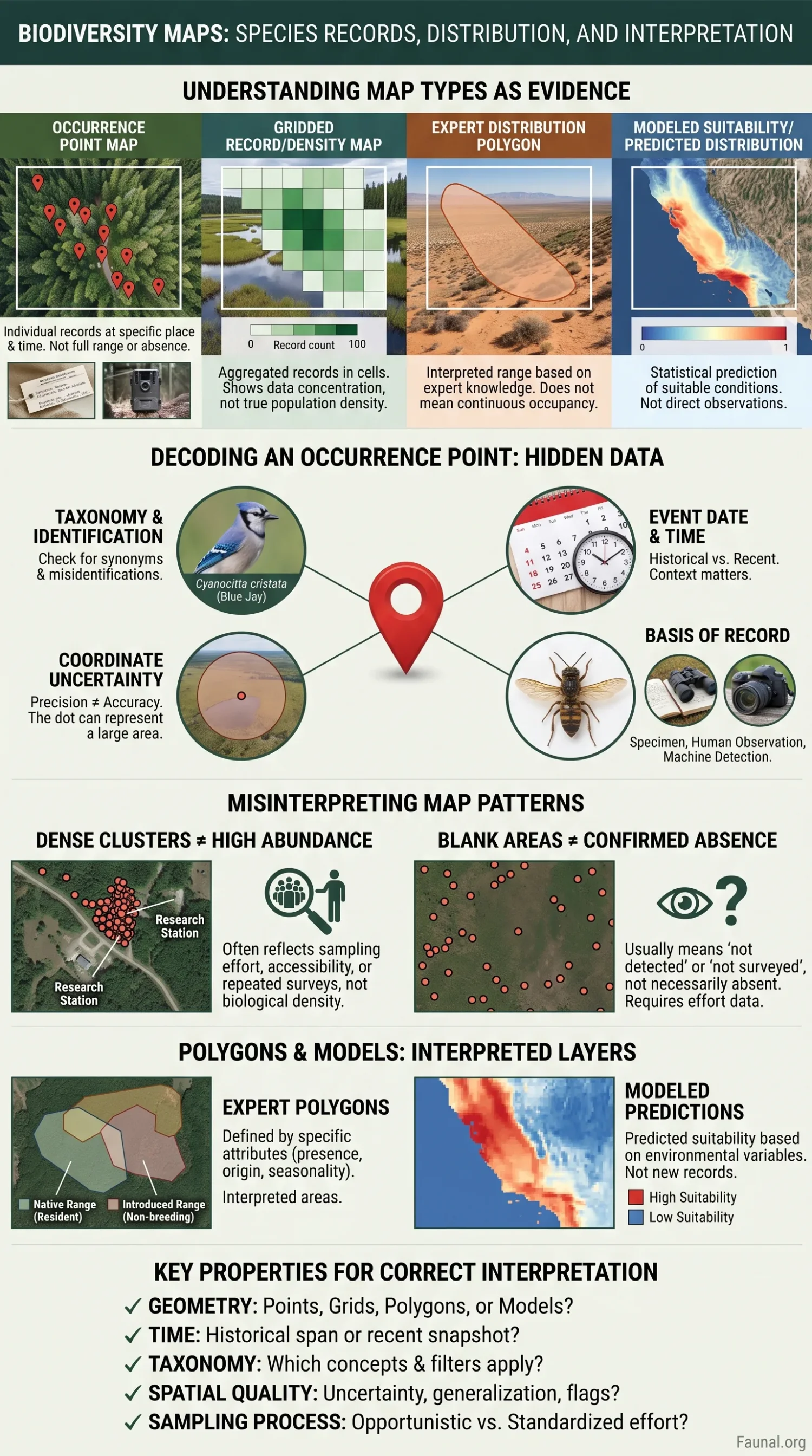
A biodiversity map can show where organisms have been recorded, where experts consider a species to occur, where records are concentrated, or where a model predicts suitable conditions. Those are different kinds of evidence. A point on a map usually documents a record associated with a place and time; it does not by itself define the boundaries of a species’ range, prove local abundance, or establish that nearby unmapped areas are unoccupied.
The Same Species Can Produce Very Different Maps
The term biodiversity map covers several spatial products that answer different biological questions. Before interpreting a pattern, the first distinction is whether the mapped geometry represents records, aggregated records, an assessed range, or a statistical prediction.
| Map form | What is mapped | What it can support | What it does not establish by itself |
|---|---|---|---|
| Occurrence point map | Individual georeferenced specimens, observations, machine detections or other occurrence records. | Documented evidence that a taxon was reported from particular locations and associated dates. | The full geographic range, abundance between points, or absence from places without points. |
| Gridded record or density map | Records aggregated into grid cells, hexagons or another spatial unit. | Where the selected dataset contains more or fewer mapped records at the chosen resolution. | True population density or species richness unless sampling effort and data coverage have been accounted for. |
| Expert distribution polygon | An area delineated from assessment data, expert knowledge, records and other spatial evidence. | A spatial representation of the assessed distribution under the definitions used by the publisher. | Continuous occupancy of every location inside the polygon. |
| Modeled suitability or predicted distribution | A statistical surface calculated from occurrences and environmental or other predictor variables. | Places predicted to have conditions associated with occurrence under the model and its assumptions. | A direct observation at every predicted location or proof that the organism is currently present there. |
A biodiversity portal may offer more than one of these products for the same taxon. The Atlas of Living Australia, for example, distinguishes occurrence-record points from expert distributions. That distinction matters because a point is a record-level object, while a distribution polygon is an interpreted spatial product.
What an Occurrence Point Actually Represents
An occurrence record is evidence associated with an organism or taxon at a place and, when available, a time. The underlying record can come from a preserved specimen, a human observation, a machine observation, a fossil, a material citation or another recognized record type. The symbol displayed on a map often hides much of this record-level information.
Two points that look identical on a map can therefore have very different evidential properties. One might represent a recent camera-trap detection with precise coordinates. Another might be a museum specimen collected a century ago and later georeferenced from a locality description covering several kilometres.
| Record field | Why it changes map interpretation |
|---|---|
| Scientific name and taxonomic status | The record must be attached to the intended taxon. Synonyms, changed classifications and identification errors can alter which points appear under a species name. |
| Basis of record | Shows the nature of the record, such as a preserved specimen, human observation or machine observation. It also helps separate wild occurrence evidence from records that may represent living collections or other contexts. |
| Event date | Places the evidence in time. A historical record and a recent record should not automatically be treated as evidence of the same present-day situation. |
| Latitude and longitude | Provide the mapped position when usable coordinates are available. |
| Coordinate uncertainty | Describes the radius around the stated coordinates within which the actual locality is expected to fall. A point symbol can therefore imply more spatial precision than the underlying record contains. |
| Occurrence status | Distinguishes detection from non-detection when that information is recorded within an appropriate event structure. |
| Data generalization or withheld information | Can indicate that published coordinates were deliberately made less precise, including cases where sensitive locality information is protected. |
Coordinate Uncertainty Extends Beyond the Dot
Darwin Core defines coordinateUncertaintyInMeters as a horizontal distance around the supplied coordinates that contains the location. A map marker may be rendered as a tiny point even when the underlying locality has uncertainty measured in hundreds or thousands of metres. The visual size of the marker is therefore not a measure of spatial accuracy.
A Precise-Looking Marker May Represent a Broad Locality
Coordinate precision, coordinate uncertainty and map-symbol size are separate properties. Extra decimal places in latitude and longitude do not prove that the original locality was recorded at that level of accuracy.
Why Record Density Is Not the Same as Animal or Plant Density
Occurrence databases combine records collected for many purposes and with very different levels of effort. Museums may hold dense historical collections from particular expeditions. Bird observations may be concentrated near roads, cities and frequently visited reserves. Camera traps can create repeated detections at fixed stations. Some countries and taxonomic groups have far more digitized data than others.
GBIF explicitly identifies unequal geographic and taxonomic sampling as a data-use problem. A dense cloud of occurrence points may partly reflect where observers worked, where institutions digitized collections, which taxa received attention, which datasets were published and which records could be georeferenced.
More mapped records do not automatically mean more individuals. Record count and biological abundance become comparable only when the data collection design, effort and observation process support that inference.
Repeated Records Can Describe Effort as Much as Presence
One locality visited every week can generate far more records than an equally suitable locality surveyed once. A grid-cell map may then show the first area as a hotspot of records even if the underlying populations are similar. Duplicate observations, repeated monitoring and dataset overlap can add another layer of record concentration that must be checked before counts are treated as ecological measurements.
Blank Areas Do Not Automatically Mean Absence
A place without occurrence points can have several explanations. The species may genuinely be absent. The area may never have been surveyed. Observations may exist but remain unpublished or ungeoreferenced. Records may be stored under another scientific name. A dataset filter may exclude older evidence. Sensitive localities may have been generalized or withheld.
Ordinary presence records are especially weak evidence for absence because they usually document where an organism was detected rather than where observers searched and failed to detect it. The missing piece is often sampling effort.
Standardized Sampling Can Support Stronger Absence Inference
Sampling-event datasets retain information about survey events, protocols and effort. When a method was designed to detect a taxon or taxonomic group, a documented non-detection can carry information that an empty area on a presence-only map cannot provide. Even then, non-detection and biological absence are not identical: detectability, season, weather, life stage and method can affect whether an organism is found.
No Point Is Not the Same as a Verified Absence
An empty map cell should be treated as missing occurrence evidence unless the underlying survey design provides a defensible basis for interpreting non-detection.
Distribution Polygons Answer a Different Spatial Question
A range or distribution polygon is not simply a collection of occurrence points joined by a line. Depending on the authority and taxon, its construction can incorporate observations, specimens, habitat information, expert assessment, known geographic barriers and other evidence.
IUCN Red List spatial data illustrate why polygon attributes matter. Red List geographic information distinguishes categories of presence, origin and seasonality. A species can be native in one part of a mapped area and introduced in another, resident in one region and present only during a breeding or non-breeding season elsewhere.
The polygon should therefore be interpreted according to the definitions and attributes supplied with that spatial dataset. Filling an area on a map does not mean that every square metre is occupied. Mountains, rivers, unsuitable vegetation, urban areas, depth limits and other ecological constraints can create unoccupied space within a broad mapped range.
Distribution, EOO and AOO Are Not Interchangeable
A species distribution map should also be kept separate from the Red List measures extent of occurrence and area of occupancy. These are geographic-range measurements used within Red List assessment procedures, not alternate names for any polygon labelled as a species range. Their calculation and biological meaning depend on defined assessment rules.
Modeled Distribution Is a Prediction Layer
Species distribution models and ecological niche models use known occurrences together with environmental variables or other predictors to estimate where conditions may be associated with a species. The result is often displayed as a continuous suitability surface or as a binary suitable/unsuitable map after a threshold is applied.
This creates information beyond the original observation points, but the new pixels are model outputs rather than new biological observations. A highly suitable pixel can lack a recorded population because the species cannot reach it, the necessary habitat structure is absent, interactions with other organisms prevent establishment, the environmental data are too coarse, or the model does not include an important ecological constraint.
The reverse problem also occurs. Models can classify occupied places as unsuitable. Threshold choice, environmental variables, study extent, background or absence data, spatial resolution and the quality of occurrence records all affect the resulting map.
Prediction Pixels Are Not Additional Occurrence Records
A modeled surface extends inference into places without observations. It should retain a clear distinction between locations where the species was recorded and locations predicted to have suitable conditions.
Time Can Change the Meaning of the Same Spatial Pattern
Occurrence records can span decades or centuries. Plotting every available record together may be useful for documenting historical evidence, but it can obscure changes in current distribution. A locality occupied in 1890 is evidence of historical occurrence even if no recent record exists there. A newly documented locality may represent range expansion, improved survey coverage, a newly digitized older specimen, taxonomic revision or simply the first published record from a place that was already occupied.
Temporal filtering therefore changes the question being asked. A map of all known records asks where occurrence has been documented across the selected record history. A map restricted to recent years asks where the selected dataset contains recent evidence. Neither one automatically measures change in population size or proves contraction or expansion without additional analysis.
Taxonomy Can Change a Map Without Any Animal Moving
Species names are another filter between raw records and mapped distribution. Historical records may use synonyms. A former species may be split into several taxa. Two names may later be treated as the same species. An identification may be revised after examination of a specimen, photograph, recording or genetic evidence.
A search using only one name string can therefore omit relevant records, while automatic name matching can sometimes bring together records created under different taxonomic concepts. Darwin Core separates fields for scientific names, accepted name usage, taxonomic status and identification information so that these relationships can be represented rather than reduced to a map label.
Unexpected outlying points deserve particular attention. They can be valuable evidence of an overlooked population, dispersal event, vagrant individual or introduction, but they can also result from misidentification, incorrect coordinates, swapped latitude and longitude, an inappropriate taxonomic match or a record from captivity.
Geospatial Flags Identify Problems, Not Automatic Deletions
Large biodiversity networks perform automated checks because coordinate errors can place records in biologically impossible locations. GBIF identifies issues including zero coordinates, coordinates outside valid latitude or longitude ranges, country-coordinate mismatches and coordinates that cannot be interpreted.
A flag is a reason to inspect the record and its intended use. It is not always proof that the biological observation itself is false. A country-coordinate mismatch, for example, could reflect a coordinate error, a country coding problem, a border issue or another data-processing problem. Record validation should consider the original information and the biological context.
Map Resolution Changes What a Pattern Appears to Say
The same records can look sparse as individual points, nearly continuous when aggregated into large grid cells, and highly clustered when displayed at finer resolution. Grid size changes the apparent continuity and density of a distribution even when the underlying occurrence dataset remains unchanged.
Spatial resolution should also be compatible with record precision. A locality with several kilometres of uncertainty cannot support metre-scale ecological inference simply because the map can zoom to that level. Historical locality descriptions and intentionally generalized sensitive-species records are common reasons for treating fine-scale patterns cautiously.
Five Properties Determine What a Biodiversity Map Can Support
- Geometry: determine whether the layer contains occurrence points, aggregated cells, polygons or modeled pixels.
- Time: check the dates represented and whether historical and recent records are being combined.
- Taxonomy: verify which taxon concept, accepted name, synonyms and identification filters are included.
- Spatial quality: consider coordinate uncertainty, georeferencing status, generalized locations and data-quality flags.
- Sampling process: establish whether the dataset contains opportunistic presence records or standardized events with information about survey method and effort.
These properties determine which ecological statements can reasonably be made from the mapped data. A recent, verified point can support local occurrence evidence. Repeated detections from standardized surveys can provide stronger evidence about use of a site. A set of opportunistic points can show the geographic pattern of available records but may not support comparisons of abundance. An assessed range polygon can represent a broader distribution while still containing areas without continuous occupancy.
What Different Map Patterns Can and Cannot Establish
A cluster of points establishes that many selected records are mapped near one another. It may reflect biological concentration, observation effort, repeated monitoring, accessibility, dataset overlap or a mixture of these influences.
An isolated point documents an outlying record if the identification and locality are reliable. It does not automatically prove a resident population or justify extending a continuous range polygon to that location.
A gap between records shows a gap in mapped evidence. Biological absence requires stronger information about survey coverage, detection and habitat.
A filled range polygon expresses the spatial interpretation used by the dataset or assessment. It does not state that organisms occupy every point within its boundary.
A high model score means the location received a high predicted value under the chosen model. It remains a prediction until supported by suitable field or occurrence evidence.
Biodiversity maps are strongest when the record type, taxonomic scope, dates, spatial uncertainty, sampling process and map geometry remain attached to the pattern being interpreted. Removing those properties can turn a map of documented evidence into an unsupported claim about complete distribution.
Sources and Verification
- GBIF — Data Quality Requirements for Occurrence Datasets — Record requirements and recommended fields for scientific names, dates, coordinates, coordinate uncertainty and occurrence data.
- TDWG — Darwin Core Quick Reference Guide — Definitions for occurrence, event, location, taxonomy, basis of record, occurrence status and coordinate uncertainty terms.
- GBIF — Occurrence Issues and Flags — Geospatial and record-processing flags used to identify common problems in occurrence data.
- GBIF — Handling Data Quality — Guidance on geographic and taxonomic sampling gaps, misidentification and data-quality checks.
- GBIF — Data Quality Requirements for Sampling-Event Datasets — Survey methods, sampling effort, events and the interpretation of detections and non-detections.
- GBIF — What Is an Ecological Niche Model? — Distinction between known occurrences and geographic predictions derived from environmental associations.
- IUCN Red List — Mapping Standards and Data Quality — Current Red List spatial-data standards, including distribution mapping and standardized spatial attributes.
- IUCN Red List — Assessment Supporting Information — Geographic-range information including presence, origin, seasonality, extent of occurrence and area of occupancy.
- Atlas of Living Australia — Species Map Layers — Operational distinction between occurrence-record points and expert distribution polygons in a national biodiversity portal.